Understanding the scattering results
The direct result of a small-angle scattering measurement is the scattering pattern, i.e. the two-dimensional image recorded by the position sensitive detector. This can be considered as a matrix of positive integer numbers, each matrix element corresponding to an image element of the sensitive surface of the detector. The numbers in the matrix elements are the total number of X-ray incidences registered by the given pixel during the time of the exposure. A typical scattering pattern is shown below.
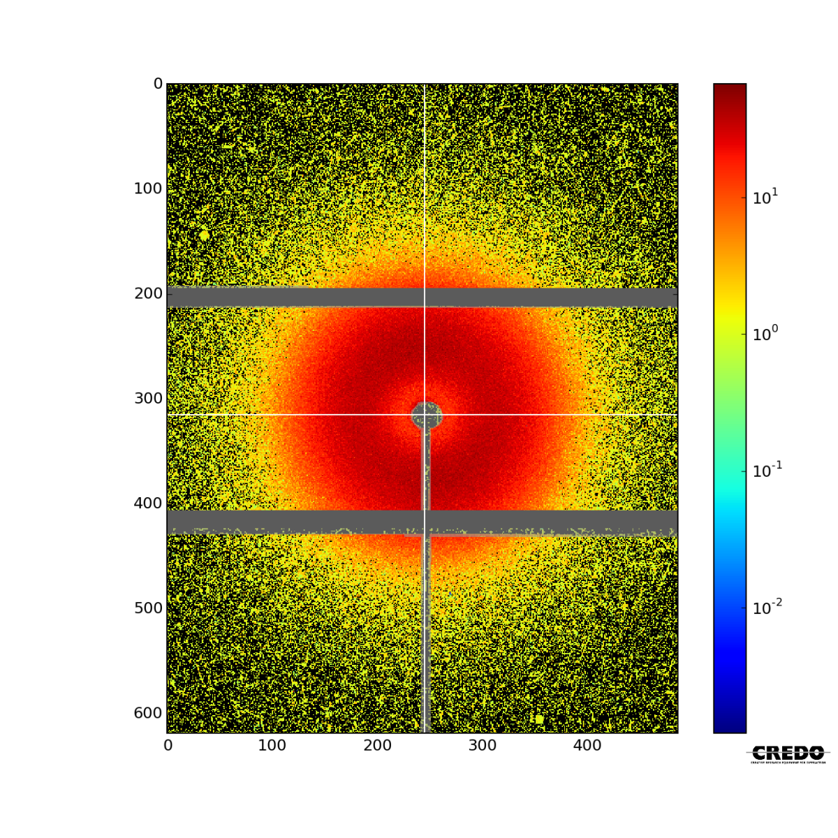
The image is a colour-coded representation of the scattering intensity matrix. The colour scale of this representation is found on the right side. The white crosshair points the position of the direct beam, aka. beam center, which is the position at which the direct, non-interacting radiation would hit the detector surface. This corresponds to $q=0$. From the definition of the scattering vector, $\vec{q}$, it is clear that the momentum transfer vectors corresponding to each point on a given circle around the beam position have the same magnitude, which is in direct relation with the radius of the circle. More precisely the following holds:
$$q=\frac{4\pi}{\lambda}\sin{\left(\frac{\tan^{-1}{\left(\frac{r}{L}\right)}}{2}\right)}\textrm{,}$$
where $r$ is the radius of the circle in real space length units, and $L$ is the sample-to-detector distance.
The grayed-out parts are called "masked": these are not taken into account by subsequent image processing and data reduction routines. Different areas of the detector might be masked because of several reasons:
- The scattering originating from the sample is shadowed by camera elements: beam-stop or its support.
- Dead (unresponsive or overresponsive) pixels
- Insensitive areas ("gaps") between detector modules
- High parasitic scattering in the region (compared to the sample scattering)
The scattered intensity can be represented in a more tractable, one dimensional form using azimuthal averaging, i.e. collecting the intensity of pixels falling into concentric rings of the scattering pattern. The following figure intends to clarify the concept.
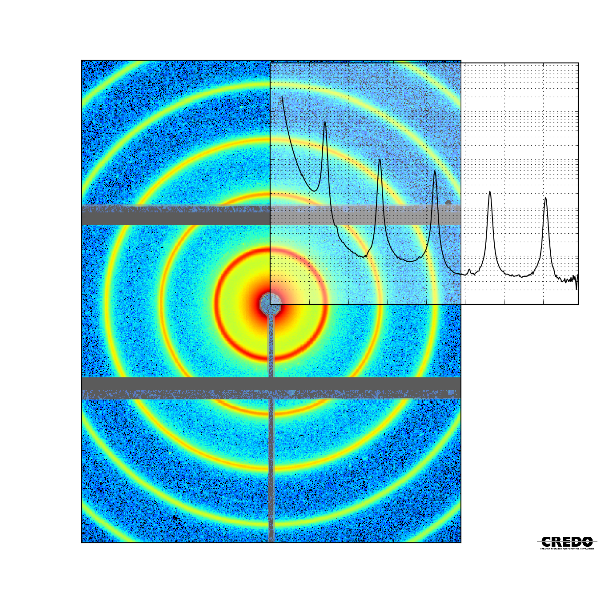
The resulting curve, the so-called radial scattering curve is more convenient to handle, plot and employ as initial dataset for model fitting.